Building a simple FM Receiver

Note: This lesson assumes you have already acquired an SDR and found a station you can receive.

In this lesson we’ll be building a basic FM Broadcast receiver and demodulator. Just as modulation is the process of varying some signal to add information to it, demodulation is the process of extracting some signal from the received signal.

FM Radio broadcasts are sometimes called Wide-band FM (WBFM), in comparison to Narrow-Band FM (NBFM) which is used in special circumstances such as emergency alerts. The goal is to build some familiarity with the tool, and understand a bit how pipelines are constructed. We’ll go much more in depth on FM radio in another lesson. In the interest of keeping this lesson (as) short (as possible), some specifics will be omitted for now.

We’ll be using GNU Radio Companion (GRC). GRC is free software, community developed, that allows you to visually build pipelines to capture radio data and transform it. It supports most SDR hardware, including RTL-SDR and HackRF One.

Go ahead and install GRC.

Now the goal for this lesson is to build a pipeline that will allow us to listen to FM radio broadcasts in GRC. Though we just did this in the previous lesson, doing so in GRC is useful for a few reasons.

1. It allows us to better understand FM radio.
2. By building the pipeline in GRC, we have more flexibility in how we use the data. While the previous tools let us listen to the signal, this wouldnt be very useful if the data were data (perhaps images) instead.

Go ahead and startup GRC, and we’ll begin building this pipeline. The analogy GRC uses for radio transformations is a bit like a flowchart. Boxes represent things that create, consume, or transform data. We then connect the inputs and outputs of these boxes to control how data flows through our pipeline.

First, we need to include the data from our SDR. At the top of GRC, there should be a magnifying lens icon. This is the best way to find blocks when you know what they’re called.

Our SDR input block is called “RTL-SDR Source”. If you just type “SDR” you should be able to find it. Then either double click it, or drag it out into the main area. You should now have a block that looks like this:

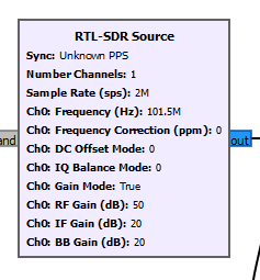
Don’t worry about the numbers, we’ll come back to configure it in a moment. First lets add a few more blocks to our pipeline. You’ll also want a “QT GUI Frequency Sink”, and a “Variable” block.

Variables, just like in math or programming, are just names we give to values. In GRC, it is convenient to use variables to avoid typing in the same value in many places. Additionally, if we want to change parameters, we can just change the value of the variable.

Lets name the variable “sample_rate”. This will represent how often the SDR should take a snapshot of the data it sees. Then go ahead and copy that variable block (select it, ctrl+c and ctrl+v as usual). Name this one “frequency”, which is the FM station we want to pick up.

Set the value for “sample_rate” to 2 million. Note that you can use scientific notation, ex: 2e6 for “2*10**6”. One thing to be aware of, is that even though GRC shows suffixes like K and M, it doesn’t actually understand these. Instead use e3 for k or thousand, and e6 for m or million.

Now set frequency to one of the stations you found previously. I’m using 101.5 FM, which is 101.5e6 in GRC.

Now lets configure our source block. Double click it to open up the editor, and copy these settings.

• Sample rate: You can just type sample_rate to use the variable you defined.
• ch0 Frequency: frequency
• ch0 RF Gain: 50
• ch0 IF Gain: 20
• ch0 BB Gain: 20 You can leave the rest of the settings as their defaults.

The little colored boxes beside our blocks represent inputs and outputs. They are color coded to represent the type of data they represent. I’ll be sure to explain any colors where they’re important. You can find more on the GRC wiki.

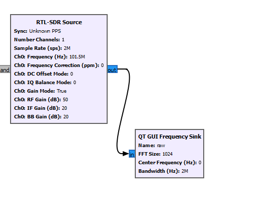
For now, it is enough to know that you need to match the colors. Connect the output from our SDR to the Frequency sink. This will let us visualize the data received right off our SDR. Configure our frequency sink. Give it a name like “raw”, and make sure to set the bandwidth to sample_rate.

It should look like this:

Now you should have no red boxes, and thus be able to run your program. Click the play icon along the top of GRC, and you should see your program in progress. You should see an animated graph that looks like this:

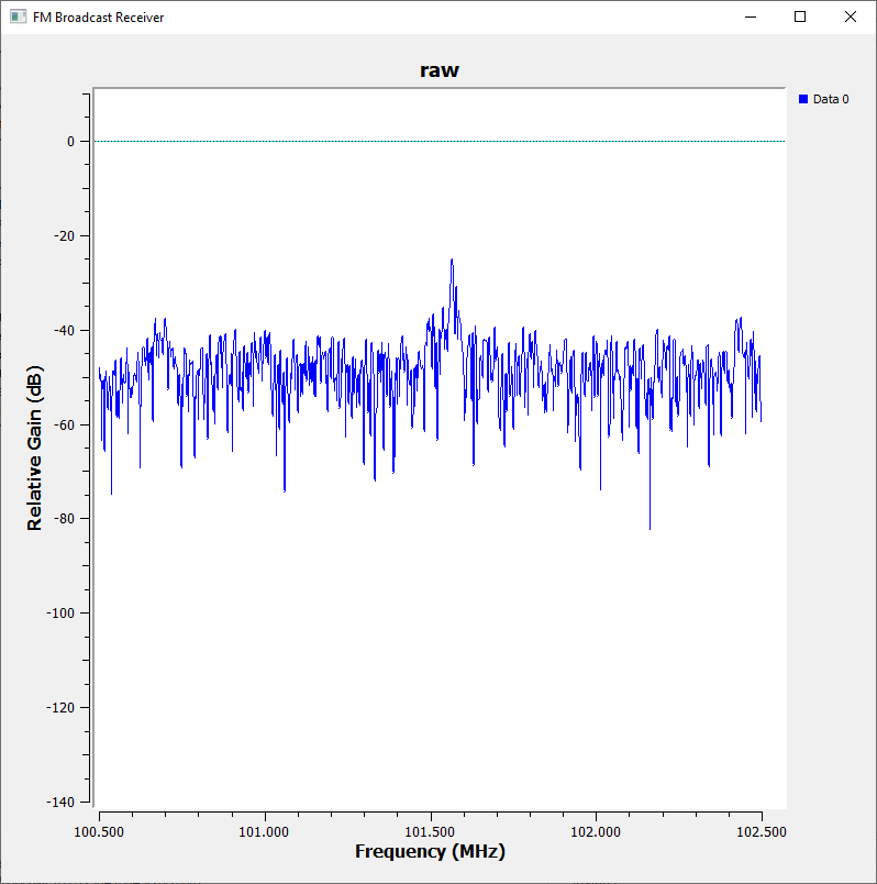
This diagram is showing us the intensity of each of the frequencies we picked up. The x axis is the various frequencies, and the Y axis is the intensity. FM signals are typically strongest around the center, so you should have a bit of a peak in the middle of your graph.

We have captured a lot of data, which includes our FM signal of interest, but also a lot of signal from neighboring frequencies. FM radio broadcasts operates on frequencies within 75khz of the ‘center frequency’, which is the station you found earlier. Anything farther away is noise. We’ll add a filtering step to drop these distant signals.

Search for and add a ‘low pass filter’ after your source. Update these settings:

• Sample rate: sample_rate
• Decimation: 10
• Cutoff freq: 75k
• Transition width: 25k

Add another “QT GUI Frequency Sink” so we can observe the filtered output. Configure it as before, but name it something like “filtered” so you can tell it apart from the other one. Connect it after the low pass filter. Run your new pipeline, and you should get something like:

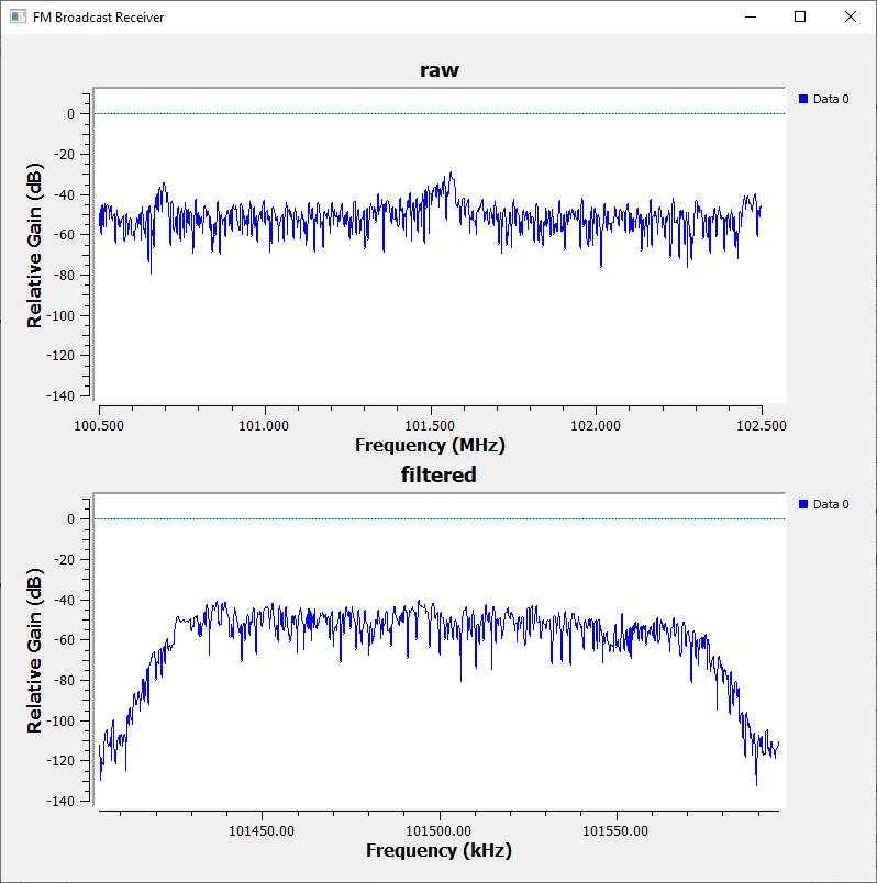
Notice how the intensity of the signals at the edges is now reduced. This is exactly what we wanted to do.

A few more blocks then we should have a working receiver + demodulator. Add these blocks:

• Rational resampler
• WBFM Receive
• Audio Sink

We’ll work backwards from the audio, since this will make the most sense.

48khz is a typical sample rate for typical audio. Just as our SDR received data by sampling constantly, speakers reproduce audio by adjusting their position many times per second.

Just before the Audio Sink, we’ll connect up the WBFM Receive. This block is what actually does the bulk of the FM decoding. In a future lesson we’ll build this ourselves, but for now we can just use it as is. The block takes two parameters, quadrature rate and audio decimation. You’ll see a decimation parameter on a bunch of blocks, and it is essentially a reduction of the data that is sent through. Decimating by 10 means that for every 10 samples that comes in, one goes out. In order to improve performance, it is best to decimate as much as possible without losing your data. Use 10 for the Audio decimation.

Since our audio sink wants 48k, use 48k*10 = 480k for the quadrature rate. Quadrature rate will also be explained more in the future.

Finally, between the WBFM receive block, and the low pass filter, we’ll want a Rational Resampler. This acts a bit like the decimation parameter we saw earlier, except that it supports fractional (rational) scaling. We’ll use 100k for decimation, and 480k for interpolation.

Now you should have a fimal diagram that looks something like this:

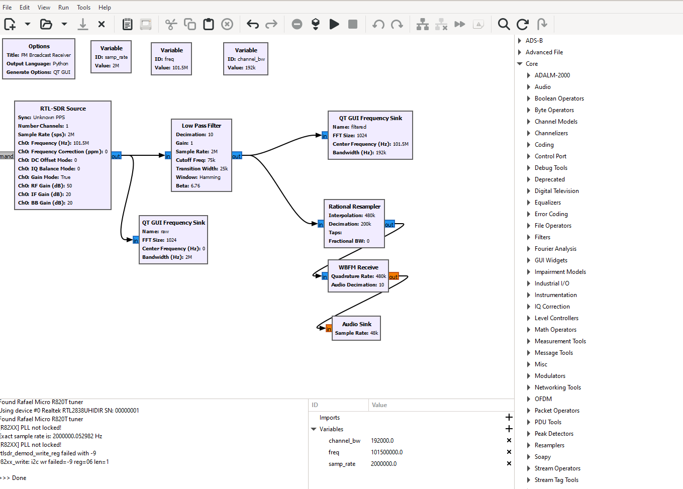
If all went well, you should be able to click play, and hear the station you selected earlier :)

If you found this article helpful, consider sharing with others that you believe would enjoy it. In a future lesson, we’ll build the WBFM decoder ourselves. But first, we’ll look at AM Broadcast radio, which while simpler to decode has some other issues.

A few suggested experiments:

• What happens if you drop the low pass filter?
• Try reducing the RF gain setting on the source, and see how this impacts the resulting noise in the audio.
• Try changing the decimation on the resampler from 100k to 200k. Listen to the resulting audio. Why do you think this happens?