Signals 101 - Sound
Radios allow us to transmit various signals over great distances. First we’ll look at audio signals. Not only is it one of the more common forms of signal, it has some appealing properties that make it good for explaining more general concepts.
Human ears measure changes in air pressure over time. When we hear sound, our ears are receiving this change in air pressure, and our brain transforms this into something we can understand.
Amplitude
Sound can be represented as a graph of this changing pressure over time. We call the intensity of the signal its r amplitude. The amplitude of a constant tone is constant. We call the intensity at each point the magnitude. Even though the amplitude of this tone is constant, its magnitude varies over time.
Here is a graph for a clean and simple note, which corresponds to the key near the middle of a piano keyboard. This is a signal with amplitude 1.
And here is the correponding audio:
Frequency
In addition to the height of a wave, we care about its width, or the spacing between two peaks of the wave. We call the number per second of the wave its “frequency”, and we measure this in hertz or hz.
The frequency of sound is particularly interesting, because this is what we interpret as the note of the sound. The middle A we graphed above is a wave with frequency 440 hz.
The next white key on the piano corresponds to a wave with frequency 493.88. Note the shape of the way is identical, besides the changed frequency. While the graphs look very similar, notice that the scales on the x axis are likely different depending on your zoom.
Domain and Range
We sometimes call the horizontal or x axis of the graph the “domain” and the vertical or y axis the range. A signal is said to map, or convert, values from the domain to values in the range.
Digitization
On digital platforms like a computer, we need to convert a smooth wave into a collection of numbers that can be represented on a computer. This is done in both directions (left/right and up/down).
Quantization
Quantization is the process of taking a smooth point from some ideal smooth waveform into a “chunkier” point more easily represented in a computer.
There are many approaches to this, but we will look at 8 bit PCM, which is one of the simpler techniques and often used for uncompressed WAV audio. For each point, the value of the signal is converted to a value between 0 and 15. These are the values that can be represented by a 8 bits in a computer.
Lets assume we have an input that ranges from -1 to +1. -1 from the input would be converted to a 0, and a +1 would be converted to 15. For all points in between, we round to the nearest whole number. The more bits used for each point, or sample, the higher the digital audio quality.
Sampling
We just discussed quantization, which is done for each point. Sampling controls of frequently we take a value from the input and turn it into an output value. An ideal “real world” signal has infinitely many points that make up the signal, and it is perfectly smooth. Digitally, we need to decide how frequently to sample the input signal.
How do you determine the right sampling rate? A key idea here is the Nyquist sampling theorem, which says that you need to sample at least two times the highest frequency of the input in order to avoid losing information. So in our earlier example, if we played a sound with A = 440hz and B = 493.88 hz, we would need to sample at least 2xB = 2x 493.88 = 987.76 times per second or hz.
The highest frequency that can be heard by humans is about 20000 hz or 20khz. CD audio is often sampled at 44.1khz, due to the sampling theorem.
Here is our A=440 hz wave again, but this time only sampled at 1320 hz.
Combining Waves
To create a sound with two notes playing at the same time, we can just add their waves together. For a digital signal, once the inputs are at the same sampling rate, each sample can just be added together. In order to keep the volume the same, each sum is usually then normalized to keep it within the original range.
Time to Frequency Domain
The time domain, where graphs are plotted vs time, is the most intuitive and also the most common way of looking at the signal. All the graphs we’ve seen so far have been in the time domain. It is also useful to look at signals in the frequency domain, to see which frequencies or notes are present in the signal at a given time.
To do this there is a technique called the Fourier (for ee aay) Transform. An efficient approach for computing this is known as the Fast Fourier Transform, or FFT. You will often see “FFT” used as the term to describe the tool to extract frequencies from audio.
The math it outside the scope of this lesson, but feel free to read up on Wikipedia if you are interested. The important piece to know for signal processing is that it is operates over smaller chunks or windows of the digital data, and tells you which frequencies are present and with what significance or magnitude.
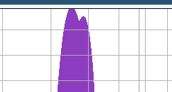
Here is a screenshot of performing the FFT on our A=440hz + B=493.88hz example signal, using the open source tool Audacity.
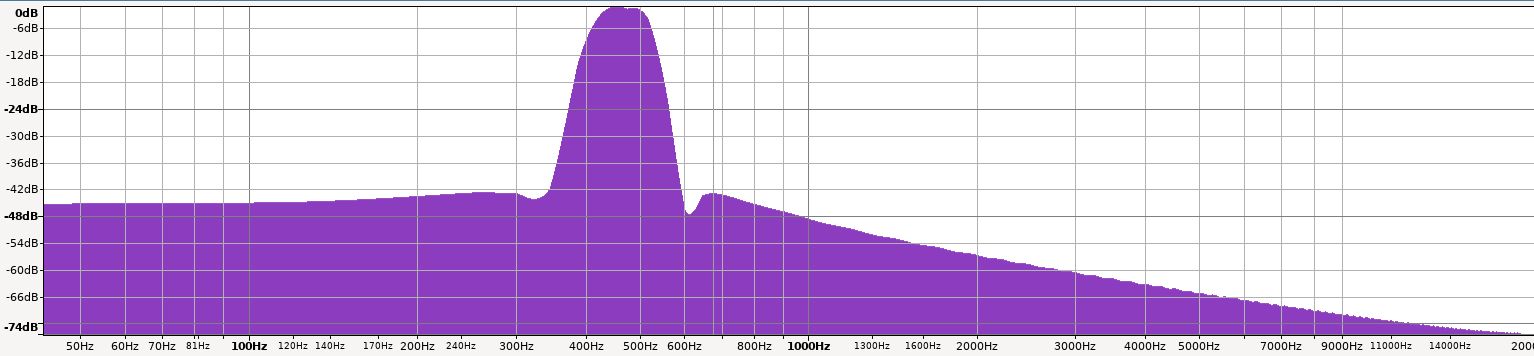
And if we zoom in, we can see the two peaks at 440hz and 498.88 hz.
#